
As my first subject for this animation blog series, we will be taking a look at Animation curves.
Curves, or better, easing curves, is one of the first concepts we are exposed to when dealing with the subject of animation in the QML space.
What are they?
Well, in simplistic terms, they are a description of an X position over a Time axis that starts in (0 , 0) and ends in (1 , 1). These curves are to be applied to a numerical property. For example, say we want to move the value of X from 0 to 250 over a time period of, say, 5000 ms in a linear fashion (constant speed), we would do something like:
NumberAnimation {
        .....
        property: "x"
        duration: 5000
        easing.type: Easing.Linear
        from:0
        to:250
        .....
    }
And it works relatively well – for reference you can see most of them here.
However there is a limited set of curves, and that poses a problem when trying to achieve more complex animation patterns, probably because no single curve in the above list reflects that complex animation we are trying to describe.
Usually the most common solution will be to reach those by using sequential and parallel animations. This creates, in my experience, a lot of trial and error code that we tend not to be particularly proud of. This is mostly because even describing simple enough animations as, say, kicking a ball that jumps, rolls, bounces and stops, requires a lot of code. We need to describe the y movement in a sequential animation, an x movement in another parallel animation and the rolling phase in yet another animation stage. The code required to generate this is big, clunky and hard to read, given the nature of multiple parallel and sequential animations running under the same master animation.
On top of that, sequential animations suffer from another, more fundamental limitation: they mostly rely on a “stop” of the motion in order to “start” the next movement when jumping from one curve to the next. Not using this will result in non continuities in the speed variation, spikes, and this will look unnatural (a non smooth speed variation indicates an infinite acceleration, and only infinitely rigid materials can achieve that when colliding with other similar materials, which doesn’t happen in nature).
The speed can be seen as the angle of the curve on each point in the chosen easing curve. The steeper the curve, the faster the movement, so when we have a sequential animation, it is important that, when transitioning from one curve to the next, the end angle of one curve is the same as the start angle for the next. Now, given the limited set of curves we are offered, we will have a hard time matching those, other than for curves that fade/start into a flat angle, aka the motion stops and restarts from one motion to the next.
How can we circumvent that limitation?
Can’t I just use my custom curves?
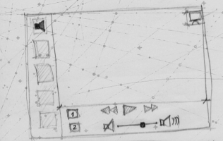
The reality is that you can, and it is relatively simple to do. Let me introduce you to the QML easing Curve Editor: one simple application that can be found in your bin Qt folder, named qmleasing. This helps you create such curves.
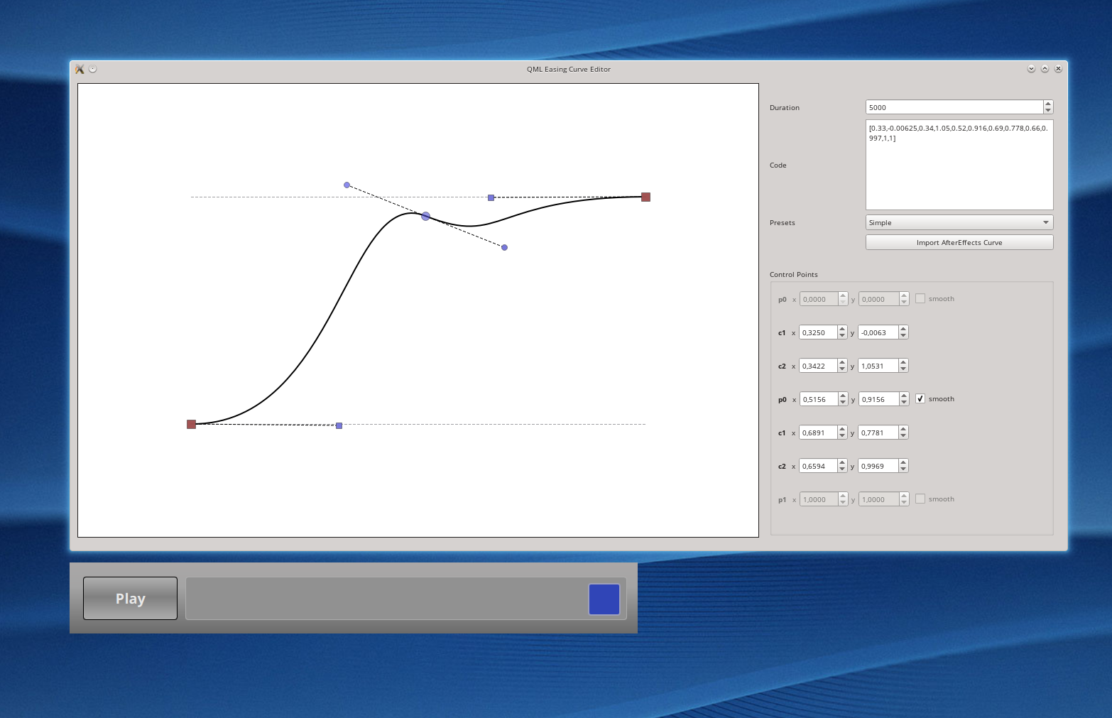
Here you can see an example of such a curve being created. Notice the ticked smooth flag that enforces that the curve is smooth at the junction of the 2 bezierCurves. This allows us to create far more complex animations, as natural as we can achieve, using this UI. The practical usage of this is achieved by copy pasting the simplified bezier description “[0.33,-0.00625,0.34,1.05,0.52,0.916,0.69,0.778,0.66,0.997,1,1]” into an easing.bezierCurve:
 NumberAnimation {
        .....
        property: "x"
        duration: 5000
        easing.bezierCurve: [0.33,-0.00625,0.34,1.05,0.52,0.916,0.69,0.778,0.66,0.997,1,1]
        from:0
        to:250
        .....
    }
The result will be something like this:
The first red square is moving according to a linear animation, and the second blue one is moving according to a, still relativity simple, new curve that we made on the qmleasing application. However, as you explore this, it quickly becomes obvious that what you win in freedom, you lose in control. The nature of the curve time/position is a bit counter-intuitive to your (at least my) thinking of position/speed.
The curve is and needs to be a description of a variable (numerical property) from an initial value (0) to a final value (1) over a time period also (0) to (1). This curve gets scaled and applied to whatever the time frame you chose in milliseconds and the start and end of the value that you are going to change, so when and if you do loop-like bezier curves, they will make no sense, as time “tends” to just move forwards… You need to think in terms of time and not speed, which means you look at the curve and divide it into multiple columns where the points in the curve represent the scaled position according to your to: and from:. In fact any animation coordination must be thought of in these terms: you look at the time an “event” occurs and map that as you see fit in the curve. Unfortunately this software lacks the visual tools to do this in a precise fashion .
but…
Hmmm, beziers I can do those.
As I was investigating this, it became obvious to me that this opened up room for serious exploitation and manipulation of mathematically/physics-based generated curves, and this will be the subject of the next post. I leave a teaser here in the form of the expected end result…
So, see you soon in the continuation of this specific subject of animation curve manipulation.
As usual leave your comments below.